Inspecting and Exploring Data – Applied Predictive Modelling (Chapter 3)
This post comprises my attempt in answering questions from the 3rd Chapter of the book, Applied Predictive Modelling. The chapter emphasises mostly on inspecting data and transforming appropriately any variables as per requirement. Nevertheless, I have also carried out some exploratory analyses of the variables with respect to the target class. The data set in question is the Glass Identification data set, and is characterised as follows:
Description
A data frame with 214 observation containing examples of the chemical analysis of 7 different types of glass (of which 1 type has not been recorded), presented through 9 different variables. The data frame contains no missing values.
Variable Information
- RI: The Refractive Index
- Na: Sodium (unit measurement: weight percent in corresponding oxide; the same unit for variables 2-9)
- Mg: Magnesium
- Al: Aluminium
- Si: Silicon
- K: Potassium
- Ca: Calcium
- Ba: Barium
- Fe: Iron
- Type:
- building_windows_float_processed
- building_windows_non_float_processed
- vehicle_windows_float_processed
- vehicle_windows_non_float_processed (none in this database)
- containers
- tableware
- headlamps
Data Inspection
We first inspect the target class — the Type variable — to see the distribution of various types of glasses. The following pie chart was obtained.
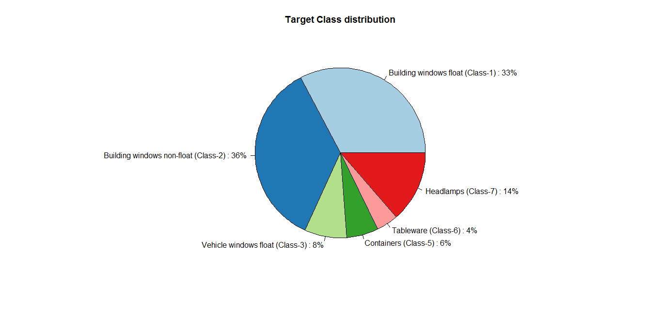
Evidently, the first two types of glasses — Building windows float and non-float — account for more than half of the total glasses. A user intending to train a classifier on this data set would, therefore, need to be cautious: any classifier trained would probably predict the first two classes better compared to other classes, such as that of Tableware.
Next, we may check whether the variables follow a normal distribution. This is essential for certain classifiers, such as Logistic Regression, which assume that variables they are being trained are normally distributed. In the following, I created a variable with normal distribution and plotted the distribution of original variables, with the intention of comparing the original variables with the normal distribution.
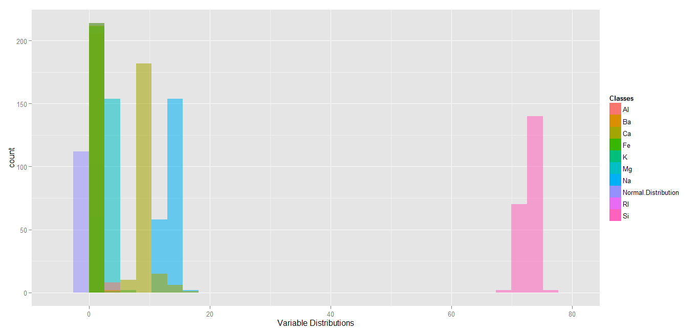
The plot shows that our variables do not follow the normal distribution. In fact, our variables are expressing different skewness and kurtosis. We may calculate both of these values for each variable: a negative skew value indicates that a variable is left skewed (and vice versa), while a negative kurtosis value indicates that a variable has a flat distribution (and vice versa).
The following plot displays each variable’s distribution, along with the respective skewness, and kurtosis. The different colours indicate our target classes as observed in each distribution.
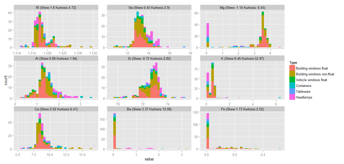
Logically, we would expect to see the first two glass types most often in the distributions, since these two were found to account for more than half of complete data set. This is apparent from the above graph: clearly, the most easily observed and large classes are the first two — Building windows float and non-float. I find the above plot to be useful for getting a ‘feel’ of the data. From this plot, we can see that, for example, the Building windows non-float has the widest range of RI, whereas the RI values for Building windows float have a relatively short range. As another example, the Mg variable can be seen to have two different groups: one containing Building windows float and Vehicle windows float, and the other containing Tableware, Containers, and Headlamps. For the Ba variable, two groups are apparent, again: one containing Tableware and another containing the rest of the variables. From all these histograms, it is clear that Building windows non-float appears to have the widest range of values, while Building windows float appears to have the tightest range.
Where the previous diagram displayed the range of values taken by each type of glass, along with the number of instances belonging to the values, the forthcoming plot stresses only the range of values.
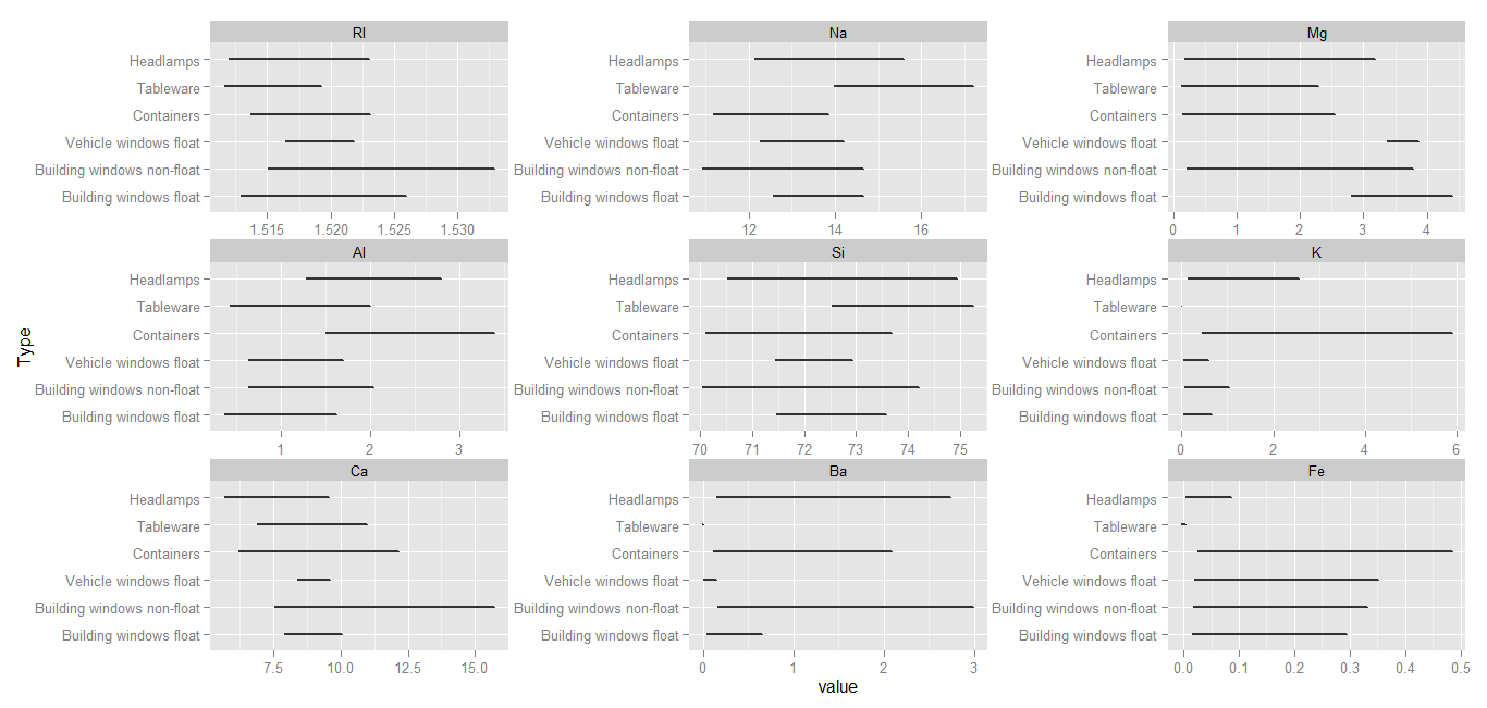
It can be observed from this plot that in case of certain variables, some glass types cover the complete range of possible values, and for others they do not. For example, Building windows non-float and Headlamps have a wide range of values for the Ba variable, implying that using Ba as a predictor for the aforementioned glass types may not be an appropriate choice. The Tableware glass type has a very tight range of values for the variables K, Ba, and Fe. This is interpreted as Tableware having very specific values for the three variables.
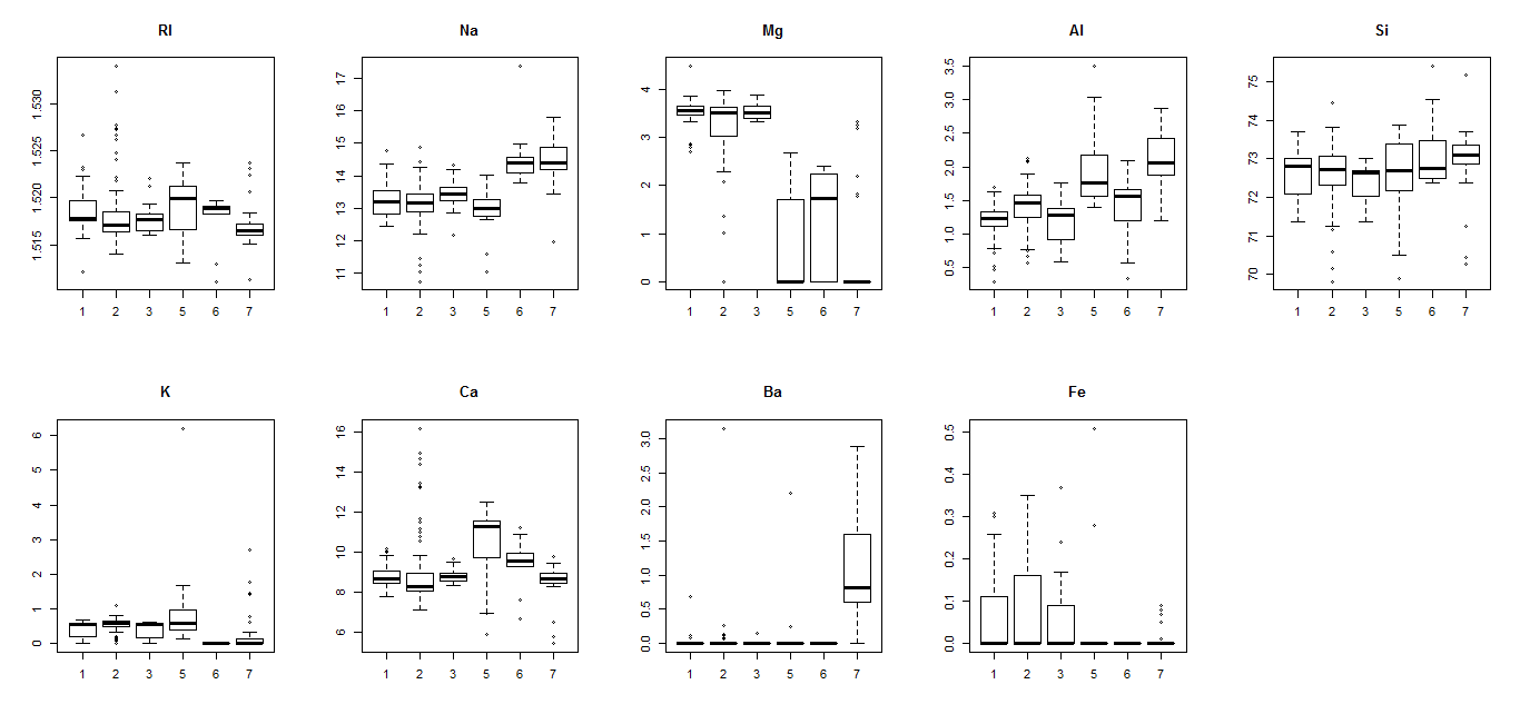
Another basic, yet effective tool for exploring data is the Boxplot. The next diagram comprises of boxplots plotted for each variable in our data frame against the target class. These compliment the histograms plot, and insights initially gleaned from histograms can be verified using these boxplots: for the variable Mg, there indeed exist two distinct groups of glass types — that of Building and Vehicle windows, and another containing Containers, Headlamps, and Tableware. Similarly, we can also verify that for the variable Ba, there appear to be two groups again, with one comprising of Tableware, and the other comprising of remaining glass types. Further inspection may reveal additional insights regarding each variable’s distribution.
A correlation matrix plot can also be used here to picture correlations between pairs of variables. A positive or negative correlation between certain variables may be noteworthy for a data analyst.
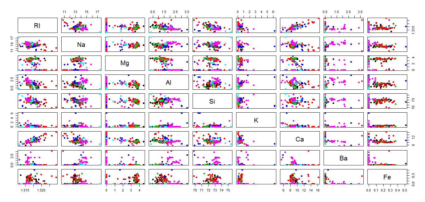
Using the plot displayed above, it can be ascertained that the Refractive Index (RI) is inversely proportional to Si and directly proportional to Ca. That is, in our glass samples, as the RI of glasses increased, an increase and a decrease were recorded in the oxide contents for Ca and Si, respectively. Further such findings may be made by studying the remaining correlations individually.
Parallel Coordinates plots may be used to discover if particular types of glass follow particular patterns, or take up specific values for each variable.
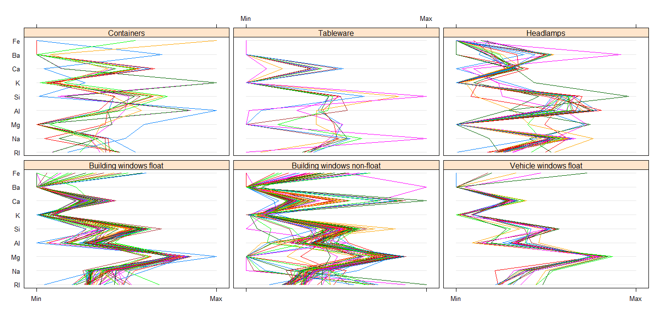
Apparently, glass types that are float processed (Building windows and Vehicle windows) follow a similar pattern for their values across variables. This may be due to the way they are processed. As well, it appears that Building windows non-float and Containers have the widest range of values for the variables.
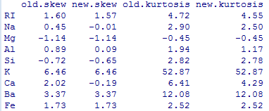
Finally, to complete our task of Data Inspection, we may want to transform specific variables, as determined by the Box Cox transformations, available from R. Once the transformations have been applied, the skewness and kurtosis of the data prior to and post transformations can be compared.
Having performed all the above inspection of my data, I feel content to conclude this post. The entire code used to perform analyses and generate graphs can be found here.