Partial dependence plots for tidymodels-based xgboost
Problem!
ML algorithms, although their proclaimed effectiveness on predictive accuracy might be suspect, are often the first tool that a data scientist resorts to when tackling a prediction problem. Such an attitude is not the best in my opinion, and I generally favour a statistical/probabilistic model over a black box1. Nevertheless, there are situations when one is asked (read: told) to use the latter.
Solution?
Then, typically xgboost is an ML model resorted to quite often, due to its good performance straight out-of-the-box. Once such a model has been trained and tested, the analyst is faced with the challenging task of explaining what the model is doing under the hood.
Problem with our solution!
To be able to explain our model — which is often more complex than to be easily explained — we tend to use techniques such as feature importance via permutation, partial dependence, and others. Notwithstanding that the 2 aforesaid techniques make an assumption of feature independence that may be unrealistic (at which point, they are not different than a vanilla regression model), such visualisations are helpful as a first attempt at model interpretation.
While working on a project, I found that some tweaks were required to be able to use the pdp package for partial dependence plots with an xgboost model built from tidymodels. Let’s try this with code that Julia Silge used in her modelling, just to quickly show the procedure.
# Load packages
pkgs <- c("tidymodels", "stringr")
sapply(pkgs, require, character.only = T)

# Read in the data from #tidytuesday repo

vb_matches <- readr::read_csv('https://raw.githubusercontent.com/rfordatascience/tidytuesday/master/data/2020/2020-05-19/vb_matches.csv', guess_max = 76000)


# Generate a derived data set for training

vb_parsed <- vb_matches %>%
  transmute(
    circuit,
    gender,
    year,
    w_attacks = w_p1_tot_attacks + w_p2_tot_attacks,
    w_kills = w_p1_tot_kills + w_p2_tot_kills,
    w_errors = w_p1_tot_errors + w_p2_tot_errors,
    w_aces = w_p1_tot_aces + w_p2_tot_aces,
    w_serve_errors = w_p1_tot_serve_errors + w_p2_tot_serve_errors,
    w_blocks = w_p1_tot_blocks + w_p2_tot_blocks,
    w_digs = w_p1_tot_digs + w_p2_tot_digs,
    l_attacks = l_p1_tot_attacks + l_p2_tot_attacks,
    l_kills = l_p1_tot_kills + l_p2_tot_kills,
    l_errors = l_p1_tot_errors + l_p2_tot_errors,
    l_aces = l_p1_tot_aces + l_p2_tot_aces,
    l_serve_errors = l_p1_tot_serve_errors + l_p2_tot_serve_errors,
    l_blocks = l_p1_tot_blocks + l_p2_tot_blocks,
    l_digs = l_p1_tot_digs + l_p2_tot_digs
  ) %>%
  na.omit()

winners <- vb_parsed %>%
  select(circuit, gender, year,
         w_attacks:w_digs) %>%
  rename_with(~ str_remove_all(., "w_"), w_attacks:w_digs) %>%
  mutate(win = "win")

losers <- vb_parsed %>%
  select(circuit, gender, year,
         l_attacks:l_digs) %>%
  rename_with(~ str_remove_all(., "l_"), l_attacks:l_digs) %>%
  mutate(win = "lose")

vb_df <- bind_rows(winners, losers) %>%
  mutate_if(is.character, factor)


# Split data for training, testing (even though we only really need the training for our purpose)

set.seed(123)
vb_split <- initial_split(vb_df, strata = win)
vb_train <- training(vb_split)
vb_test <- testing(vb_split)


# Fitting our xgboost model

xgb_spec <- boost_tree(
  trees = 1000,
  tree_depth = 4,
  min_n = 25,
  loss_reduction = 0.0011,
  sample_size = 0.977,
  mtry = 5,
  learn_rate = 0.0195,
) %>%
  set_engine("xgboost") %>%
  set_mode("classification") %>%
  fit(win ~ ., data = vb_train)
So far, so good. Now, we want to obtain partial dependence plots. The partial function from pdp expects an xgb.Booster object, along with the training data used in modelling.
pdp::partial(
  xgb_spec$fit,
  pred.var = "kills",
  ice = T,
  center = T,
  plot = T,
  alpha = .1,
  plot.engine = "ggplot2",
  train = vb_train %>% select(-win)
)
#> Error in predict.xgb.Booster(object, newdata = newdata, reshape = TRUE,  : Feature names stored in `object` and `newdata` are different!
Hmm…How are the names different?
xgb_spec$fit$feature_names
#> [1] "circuitAVP"   "circuitFIVB"  "genderM"      "genderW"      "year"         "attacks"
#> [7] "kills"        "errors"       "aces"         "serve_errors" "blocks"       "digs"

names(vb_train %>% select(-win))
#> [1] "circuit"      "gender"       "year"         "attacks"      "kills"        "errors"
#> [7] "aces"         "serve_errors" "blocks"       "digs"
Well, this is understandable, because:
- xgboost expects all categorical variables to be one-hot encoded
- tidymodels rather helpfully does this automatically for us during fitting
- since vb_train is left as is/incompatible with how xgboost sees it, the
partialfunction exits with an error
We can try adding a dummy coding step in our recipe…
vb_recipe <- recipe(win ~., data = vb_train) %>%
  step_dummy(all_nominal(),-all_outcomes(), one_hot = T) %>%
  prep()
vb_train_2 <- juice(vb_recipe)
Are the names identical now?
vb_train_2 %>% select(-win) %>% names()
#> [1] "year"         "attacks"      "kills"        "errors"       "aces"         "serve_errors"
#> [7] "blocks"       "digs"         "circuit_AVP"  "circuit_FIVB" "gender_M"     "gender_W"
Oops. Seems like the only difference now is in the underscore that separates a categorical variable from its value in our train dataset, while the model does not have any underscore separation.
Luckily, without much changes, we can get this sorted: the step_dummy function has an argument naming, which uses a function dummy_names. This function can be used to indicate whether an underscore or any other separator is to be added for one-hot encoded variables.
Below, I will create another version of this function, without any separator, and pass it to the step_dummy function.
# Creating another version of the dummy names function

dummy_names_2 <- function (var, lvl, ordinal = FALSE, sep = "")
{
    if (!ordinal)
        nms <- paste(var, make.names(lvl), sep = sep)
    else nms <- paste0(var, names0(length(lvl), sep))
    nms
}


# Testing it now

vb_recipe <- recipe(win ~., data = vb_train) %>%
  step_dummy(all_nominal(),-all_outcomes(), one_hot = T, naming = dummy_names_2) %>%
  prep()
vb_train_2 <- juice(vb_recipe)

all(vb_train_2 %>% select(-win) %>% names() %in% xgb_spec$fit$feature_names)
#>[1] TRUE
Perfect! Can we generate a partial dependence plot now?
pdp::partial(
  xgb_spec$fit,
  pred.var = "kills",
  ice = T,
  center = T,
  plot = T,
  alpha = .1,
  plot.engine = "ggplot2",
  train = vb_train_2 %>% select(-win)
)

#> Error in predict.xgb.Booster(object, newdata = newdata, reshape = TRUE,: Feature names stored in `object` and `newdata` are different!
This was strange, so I had to do a bit of debugging with traceback() to find out why this was happening. The problem seemed to be occurring at the following function within partial.
object <- xgb.Booster.complete(object, saveraw = FALSE)
if (!inherits(newdata, "xgb.DMatrix"))
  newdata <- xgb.DMatrix(newdata, missing = missing)
if (!is.null(object[["feature_names"]]) && !is.null(colnames(newdata)) &&
    !identical(object[["feature_names"]], colnames(newdata)))            # Herein lies the problem!
  stop("Feature names stored in `object` and `newdata` are different!")
It seems like identical() expects character vectors to follow the same order too, in addition to just being the same vectors:
a1 <- letters[1:5]
a1
#> [1] "a" "b" "c" "d" "e"

a2 <- letters[sample(x = 1:5, size = 5)]
a2
#> [1] "c" "a" "d" "b" "e"

identical(a1, a2)
#> FALSE

a3 <- a2[order(match(a2, a1))]
a3
#> [1] "a" "b" "c" "d" "e"

identical(a1, a3)
#> TRUE
So if we just rearrange our columns in training data in accordance with feature names of xgboost model, it should work…
pdp::partial(
  xgb_spec$fit,
  pred.var = "kills",
  ice = T,
  center = T,
  plot = T,
  alpha = .1,
  plot.engine = "ggplot2",
  train = vb_train_2 %>%
  select(-win) %>%
  select(match(xgb_spec$fit$feature_names, vb_train_2 %>% select(-win) %>% names()))
)
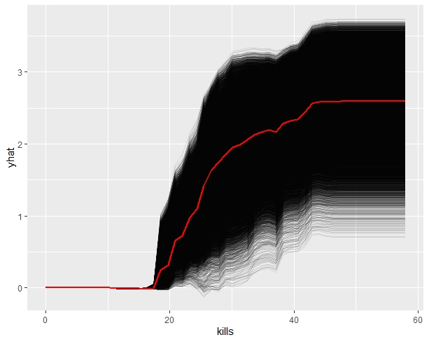
Finally!
-
If you are interested in weighing which option to choose — ML or Statistical model, here is a great resource that presents a roadmap view to select the type of modelling adequate for your problem. ↩