Feature Leakage, and the case to identify it with EDA vs. Machine Learning
This is a corrected version of an earlier post on the same topic. This version contains the correct links to the original post, to faciliate discussion via comments.
On one of my projects, my team and I were tasked with building a mortgage leads generation model for a client — a quite standard project in the banking industry. The data shared with us, on the other hand, were not safe or fit for modelling straightaway: the data had been compiled from different sources, “possibly from different time periods” too.
This might seem like an exceptional situation. In reality, however, it is all too common to acquire data from the client and take for granted their fitness for modelling. In our situation, the comment from our client meant that we were potentially looking at feature leakage.
Feature and data leakage
There are many examples of feature and data leakage, not only in corporate environments but also in competitions such as those offered by Kaggle. A future post on this blog will delve deeper into leakage, the ways it might be creep into data, and how it can jeopardise analyses and modelling. In our case, there was a danger of feature leakage: the customer account balances were suspected of including the loan amounts. They were appended to the main dataset from a time after customers had acquired a mortgage (and such mortgages are deposited into the customer’s account after acquisition, so the account balances were inflated). To add a further difficulty, the account balances had been discretised. This is very problematic on its own, as the discretisation is often arbitrary, assumes a flat relationship between the discretised feature and the target variable within the intervals, and results in loss of precision. There are various other reasons too that should deter any analyst from considering discretisation.
Feature leakage inspection - EDA vs. ML
While we shared our concerns with the data provider regarding leakage and discretisation, we also began inspecting the data to see how we might identify feature leakage. Our data comprised of customers who had obtained a loan and those who had not. A natural next step would be to do an EDA/Statistical analyses to explore how much of the leakage can be affirmed/negated.
That is when a team members suggested to instead build a simple tree-based model - any ‘leaky’ features would rank highest in variable importance. This sounded like an idea, except that it was too informal and ‘hack-like’. In such situations, it is preferable instead to adopt a formal approach.
So, is the approach of developing a quick model worthwhile to check leakage?
While there is some merit in the suggestion (especially due to the feature selection process in random forests), generally I feel otherwise because of the following reasons:
- It is unclear what threshold to use such that variable importance beyond it would signify leakage. Afterall,
- It is also not obvious how low the importance of other variables should be in comparison to another potential leaky variable.
- Feature leakage is associated more with surprisingly good predictive performance, rather than merely inflated variable importance. This means one ought to still obtain a new, unseen dataset in order to check the model’s generlisation power for evidence of leakage.
- An ML model might be a quick way to try to inspect leakage, yet it is a model afterall (and a blackbox one). In contrast to EDA or a Statistical test, it is an indirect method for inspection.
Nevertheless, I decided to use both modelling and EDA or a *Statistical test. Results of these are shown in what follows1.
Approach 1: Feature leakage identification with ML
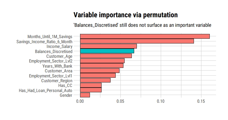
I built a quick random forest, without any bells or whistles, to see if it gave unduly high importance to the discretised balances feature.
Nothing stands out of the ordinary here. We would have expected the discretised balances to rank the highest, which it is clearly not.
Approach 2: Feature leakage identification with EDA
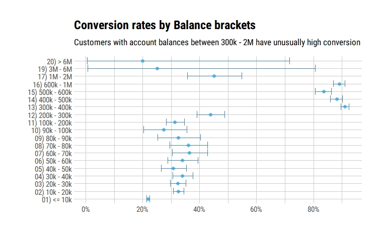
Sometimes, simply looking at the data is more enlightening than studying it via blackbox models. Following is a graph of the proportion of customers, within each discretised account balance range, who acquired a mortgage. Curiously, the proportion of customers who acquired a mortgage with account balances between 300k and 1M is extremely high (more than ~80%), whereas proportion of those with lesser account balances is steady between 20% - 30%. This increased our suspicion further, as the value of house loans in our geography is generally between 300k - 1M.
It was easy to have a discussion with our data provider with such readily digestible evidence in hand. Subsequently, we reached an agreement to have another “clean” version of the data.
This graph clearly showed an oddity in our dataset that could not be explained by the data provider. As such, it would seem there was no need for a formal statistical test then. The 1st approach had not been useful in our case, as much as I appreciated my ML colleague’s suggestion (having a ML background myself, the lure of ML is understandable). But I have gravitating slowly towards Statistics myself, for its more principled and nuanced approach to estimation and uncertainty.
And I could not waste this opportunity of testing a Statistical approach to the problem at hand…
Approach 3: Feature leakage identification with Hypothesis tests
Expressing our question into a quantitative/Statistical form was quite difficult for me:
- What should be the null hypothesis, precisely?
- How should we model the data generating process for the null hypothesis?
The first question determines how you can answer the second one. Moreover, there are (at least?) two different null hypotheses that you can test:
- That the proportion of customers who acquired a loan monotonically decreases with increasing account balance (after all, richer people do not tend to need loans as much as less rich people)
- That the number of customers who acquired a loan and whose balances do not include loan amounts follow an expected distribution (and the number of such customers decreases with increasing account balance)
I initially could only posit the 1st hypothesis, and I had to approach people with a much better understanding of Statistics than I currently have. My discussion with one such person helped me see the 2nd hypothesis. What follows below is the approach they kindly shared to carry out a Statistical test, positing a geometric distribution for the number of customers acquiring loans with increasing account balances.
library(tidyverse)

# Loading some data

loan_data <- structure(list(finalClass = c("Reject/Cancel", "Success", "Reject/Cancel",
"Success", "Success", "Reject/Cancel", "Reject/Cancel", "Success",
"Reject/Cancel", "Success", "Reject/Cancel", "Success", "Reject/Cancel",
"Success", "Success", "Reject/Cancel", "Success", "Reject/Cancel",
"Reject/Cancel", "Success", "Reject/Cancel", "Success", "Reject/Cancel",
"Success", "Success", "Reject/Cancel", "Reject/Cancel", "Success",
"Success", "Reject/Cancel", "Success", "Reject/Cancel", "Success",
"Reject/Cancel", "Reject/Cancel", "Success", "Reject/Cancel",
"Reject/Cancel", "Success"), balance_new_bracket = c("01. <= 10k",
"01. <= 10k", "02. 10k - 20k", "02. 10k - 20k", "03. 20k - 30k",
"03. 20k - 30k", "04. 30k - 40k", "04. 30k - 40k", "05. 40k - 50k",
"05. 40k - 50k", "06. 50k - 60k", "06. 50k - 60k", "07. 60k - 70k",
"07. 60k - 70k", "08. 70k - 80k", "08. 70k - 80k", "09. 80k - 90k",
"09. 80k - 90k", "10. 90k - 100k", "10. 90k - 100k", "11. 100k - 200k",
"11. 100k - 200k", "12. 200k - 300k", "12. 200k - 300k", "13. 300k - 400k",
"13. 300k - 400k", "14. 400k - 500k", "14. 400k - 500k", "15. 500k - 600k",
"15. 500k - 600k", "16. 600k - 1M", "16. 600k - 1M", "17. 1M - 2M",
"17. 1M - 2M", "18. 2M - 3M", "19. 3M - 6M", "19. 3M - 6M", "20. > 6M",
"20. > 6M"), N = c(18232L, 5115L, 1697L, 819L, 364L, 761L, 476L,
245L, 308L, 137L, 210L, 108L, 155L, 89L, 77L, 137L, 52L, 108L,
103L, 39L, 569L, 260L, 233L, 182L, 1597L, 156L, 109L, 817L, 590L,
116L, 817L, 100L, 51L, 62L, 9L, 1L, 3L, 4L, 1L), percent = c(0.780914036064591,
0.219085963935409, 0.674483306836248, 0.325516693163752, 0.323555555555556,
0.676444444444444, 0.660194174757282, 0.339805825242718, 0.692134831460674,
0.307865168539326, 0.660377358490566, 0.339622641509434, 0.635245901639344,
0.364754098360656, 0.35981308411215, 0.64018691588785, 0.325,
0.675, 0.725352112676056, 0.274647887323944, 0.686369119420989,
0.313630880579011, 0.56144578313253, 0.43855421686747, 0.911009697661152,
0.0889903023388477, 0.117710583153348, 0.882289416846652, 0.835694050991501,
0.164305949008499, 0.890948745910578, 0.109051254089422, 0.451327433628319,
0.548672566371681, 1, 0.25, 0.75, 0.8, 0.2), tots = c(23347L,
23347L, 2516L, 2516L, 1125L, 1125L, 721L, 721L, 445L, 445L, 318L,
318L, 244L, 244L, 214L, 214L, 160L, 160L, 142L, 142L, 829L, 829L,
415L, 415L, 1753L, 1753L, 926L, 926L, 706L, 706L, 917L, 917L,
113L, 113L, 9L, 4L, 4L, 5L, 5L), conf_low = c(0.775552136317493,
0.213794081502295, 0.65578046562415, 0.307220804467065, 0.296264735635882,
0.648227521218143, 0.624326658051425, 0.305255642604346, 0.646947176024304,
0.265253980427813, 0.60544358384926, 0.287709357961987, 0.571443652323727,
0.304282016481803, 0.295522603420615, 0.571952527712148, 0.25317409400087,
0.596551368545636, 0.64420157566435, 0.203150823708409, 0.653560936603063,
0.282154345692913, 0.51220524670192, 0.390195953557052, 0.896698056863425,
0.076072772673856, 0.0976559949418072, 0.859767702403072, 0.80626156910148,
0.137713232814479, 0.868959355941994, 0.0896127959455879, 0.357541357583628,
0.452272456810347, 0.663732883120057, 0.00630946320970987, 0.194120449683243,
0.283582063881911, 0.00505076337946806), conf_hi = c(0.786205918497705,
0.224447863682507, 0.692779195532935, 0.34421953437585, 0.351772478781857,
0.703735264364118, 0.694744357395654, 0.375673341948575, 0.734746019572187,
0.353052823975696, 0.712290642038013, 0.39455641615074, 0.695717983518197,
0.428556347676273, 0.428047472287852, 0.704477396579385, 0.403448631454364,
0.74682590599913, 0.796849176291591, 0.35579842433565, 0.717845654307087,
0.346439063396937, 0.609804046442948, 0.48779475329808, 0.923927227326144,
0.103301943136575, 0.140232297596928, 0.902344005058193, 0.862286767185521,
0.19373843089852, 0.910387204054412, 0.131040644058006, 0.547727543189653,
0.642458642416372, 1, 0.805879550316757, 0.99369053679029, 0.994949236620532,
0.716417936118089)), row.names = c(NA, -39L), class = "data.frame")

observed_n_per_cat <-
  loan_data %>%
  filter(finalClass == "Success") %>%
  pull(tots)

geom_negloglikelihood = function(logit_prob, dat) {
  -sum(dgeom(seq_along(dat)-1, prob = plogis(logit_prob), log = T) * dat)
}

mle_prob =
  plogis(optimize(f = geom_negloglikelihood, dat = observed_n_per_cat, lower = -10, upper = 10)$minimum)

expected_n_per_cat =
  sum(observed_n_per_cat) * dgeom(seq_along(observed_n_per_cat)-1, prob = mle_prob)

chisq_statistic <-
  sum((observed_n_per_cat - expected_n_per_cat)^2 / expected_n_per_cat)

pchisq(chisq_statistic, df = length(observed_n_per_cat) - 1, lower = F)
And so, we have a very tiny p-value, indicating that the data we have (or data more extreme than these) are very surprising, if we assume they follow a geometric distribution.
Summary
This was a very exciting opportunity to test multiple ideas:
- Can we use ML models to identify feature leakage?
- How much more effective and intuitive is EDA to identify such leakage?
- How can we express our hypothesis on potential feature leakages for Statistical tests?
Of course, EDA would be effective to identify leakage as long as it occurs in a relatively trivial fashion. More complex leakages would require complex EDA, and perhaps hypothesis testing could, then, only be the solution.
As for using ML models, I remain skeptical…
How would you formulate a hypothesis for a Statistical test, in this instance?
Do you think a better ML modelling strategy could have been used here?
All comments and critique are welcome!
-
data have been re-generated from the same distribution as found in the original situation ↩

