Bootstrap confidence intervals and confidence distritbutions - application on X-men data using ggdist
Background
Back in June, Julia Silge analysed the uncanny X-men comic book series. If, perchance, you are not familiar with her work, check out her blog and Youtube screencasts - invaluable resources for when I want to learn about any new tidyverse packages!
In her analyses of X-men comic series data from #tidytuesday, she proceeded to generate bootstrap confidence intervals for parameters of a logistic regression model. This is a very convenient way to show the variability in model parameters, but there is another package around — ggdist — that allows estimating and visualising confidence distributions around parameter estimates, in addition to several other visualisations such as the eye plot from the inimitable David Spiegelhalter.
But what is a confidence distribution?
It is a distribution estimator, like the bootstrap, but is more general than it and subsumes it. It can be thought of as a (sample dependent) distribution for all levels of a parameter’s confidence intervals, at different levels of probability. As such, it can be used, then, to also calculate confidence/compatibility intervals1, statistical power, p-values, etc.
I incline towards frequentism for most analytical problems, and the classic interpretation of confidence/compatibility distribution could pose a problem because under the frequentist view, parameters are fixed (while under Bayesian view, parameters are not fixed). In other words, previously a confidence distribution was interpreted as a distribution of the parameter. The modern definition, as outlined in this paper from Min-ge Xie and Kesar Singh, imposes certain requirements on the confidence distribution (to ensure adherence to frequentist properties), finally interpreting the distribution as an estimator for the parameter. This also means that there can be different confidence distributions that may be good, bad, worse, or best fit for a parameter of interest.
Connection to Bootstrap
Xie and Singh also note in the aforesaid paper that a bootstrap distribution is “often an (asymptotic) confidence distribution”, and a CD random variable generated from a confidence/compatibility distribution is related to and has similar theoretical properties as a bootstrap estimator.
Let’s regenerate Julia’s models/visualisations and compare it with our confidence distribution.
Bootstrapped parameter estimates
extrafont::loadfonts(device = "win")
library(tidyverse)
character_visualization <- readr::read_csv("https://raw.githubusercontent.com/rfordatascience/tidytuesday/master/data/2020/2020-06-30/character_visualization.csv")
xmen_bechdel <- readr::read_csv("https://raw.githubusercontent.com/rfordatascience/tidytuesday/master/data/2020/2020-06-30/xmen_bechdel.csv")
locations <- readr::read_csv("https://raw.githubusercontent.com/rfordatascience/tidytuesday/master/data/2020/2020-06-30/locations.csv")
per_issue <- character_visualization %>%
group_by(issue) %>%
summarise(across(speech:depicted, sum)) %>%
ungroup()
x_mansion <- locations %>%
group_by(issue) %>%
summarise(mansion = "X-Mansion" %in% location)
locations_joined <- per_issue %>%
inner_join(x_mansion)
library(tidymodels)
set.seed(123)
boots <- bootstraps(locations_joined, times = 1000, apparent = TRUE)
boot_models <- boots %>%
mutate(
model = map(
splits,
~ glm(mansion ~ speech + thought + narrative + depicted,
family = "binomial", data = analysis(.)
)
),
coef_info = map(model, tidy)
)
boot_coefs <- boot_models %>%
unnest(coef_info)
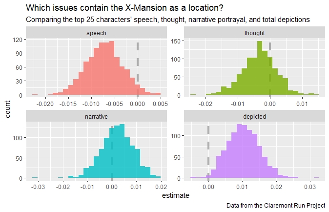
boot_coefs %>%
filter(term != "(Intercept)") %>%
mutate(term = fct_inorder(term)) %>%
ggplot(aes(estimate, fill = term)) +
geom_vline(
xintercept = 0, color = "gray50",
alpha = 0.6, lty = 2, size = 1.5
) +
geom_histogram(alpha = 0.8, bins = 25, show.legend = FALSE) +
facet_wrap(~term, scales = "free") +
labs(
title = "Which issues contain the X-Mansion as a location?",
subtitle = "Comparing the top 25 characters' speech, thought, narrative portrayal, and total depictions",
caption = "Data from the Claremont Run Project"
)
Confidence/Compatibility distribution based parameter estimates
library(ggdist)
library(hrbrthemes)

model1 <- glm(mansion ~ speech + thought + narrative + depicted,
        family = "binomial", data = locations_joined)

model1 %>%
  broom::tidy() %>%
  filter(term != "(Intercept)") %>%
  ggplot(aes(y = term, fill = term)) +
  stat_dist_halfeye(
    aes(dist = "student_t", arg1 = df.residual(model1), arg2 = estimate, arg3 = std.error)) +
  geom_vline(xintercept = 0, color = "gray50", alpha = 0.6, lty = 2, size = 1.5) +
  scale_x_continuous(breaks = scales::pretty_breaks(n = 10)) +
  labs(x = "", y = "", fill = "Term", title = "Confidence distribution for model parameters") +
  ggthemes::scale_fill_few() +
  theme_ipsum_rc(grid = "XY", axis = "xy") +
  theme(legend.position = "none")
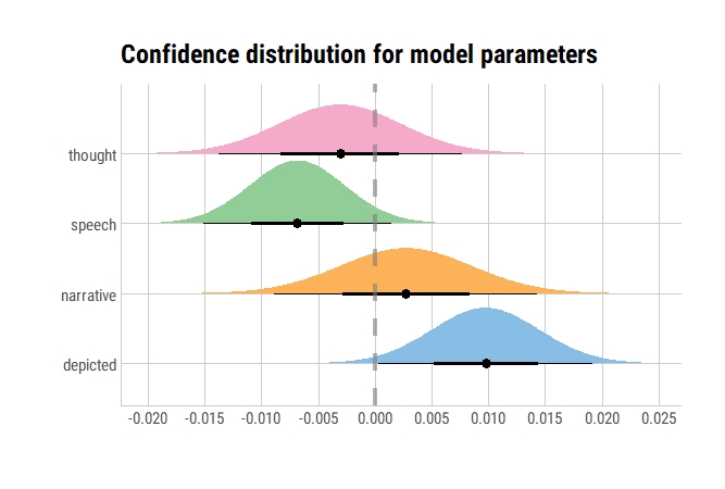
Very similar, if not exactly the same!
bechdel_joined <- per_issue %>%
inner_join(xmen_bechdel) %>%
mutate(pass_bechdel = if_else(pass_bechdel == "yes", TRUE, FALSE))
set.seed(123)
boots <- bootstraps(bechdel_joined, times = 1000, apparent = TRUE)
boot_models <- boots %>%
mutate(
model = map(
splits,
~ glm(pass_bechdel ~ speech + thought + narrative + depicted,
family = "binomial", data = analysis(.)
)
),
coef_info = map(model, tidy)
)
boot_coefs <- boot_models %>%
unnest(coef_info)
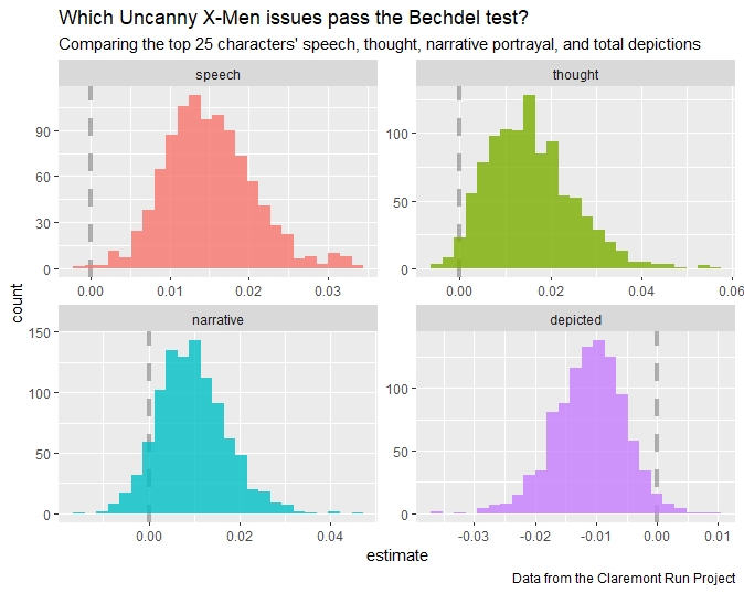
boot_coefs %>%
filter(term != "(Intercept)") %>%
mutate(term = fct_inorder(term)) %>%
ggplot(aes(estimate, fill = term)) +
geom_vline(
xintercept = 0, color = "gray50",
alpha = 0.6, lty = 2, size = 1.5
) +
geom_histogram(alpha = 0.8, bins = 25, show.legend = FALSE) +
facet_wrap(~term, scales = "free") +
labs(
title = "Which Uncanny X-Men issues pass the Bechdel test?",
subtitle = "Comparing the top 25 characters' speech, thought, narrative portrayal, and total depictions",
caption = "Data from the Claremont Run Project"
)
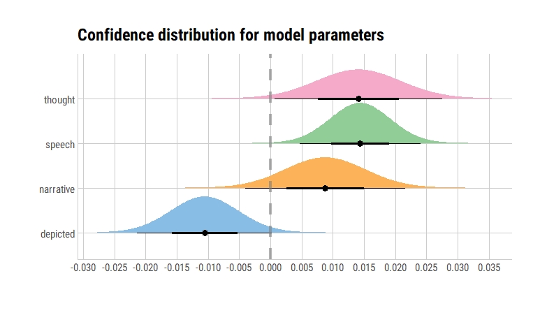
Versus…
model2 <- glm(pass_bechdel ~ speech + thought + narrative + depicted,
        family = "binomial", data = bechdel_joined)

model2 %>%
  broom::tidy() %>%
  filter(term != "(Intercept)") %>%
  ggplot(aes(y = term, fill = term)) +
  stat_dist_halfeye(
    aes(dist = "student_t", arg1 = df.residual(model1), arg2 = estimate, arg3 = std.error)) +
  geom_vline(xintercept = 0, color = "gray50", alpha = 0.6, lty = 2, size = 1.5) +
  scale_x_continuous(breaks = scales::pretty_breaks(n = 10)) +
  labs(x = "", y = "", fill = "Term", title = "Confidence distribution for model parameters") +
  ggthemes::scale_fill_few() +
  theme_ipsum_rc(grid = "XY", axis = "xy") +
  theme(legend.position = "none")
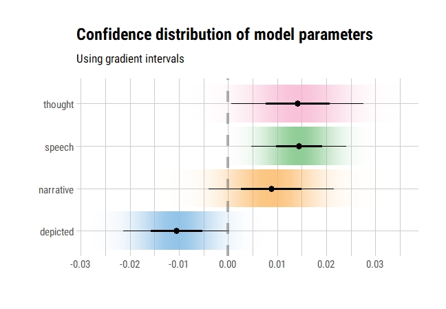
An alternative way of presenting this would be as follows:
model2 %>%
  broom::tidy() %>%
  filter(term != "(Intercept)") %>%
  ggplot(aes(y = term, fill = term)) +
  stat_dist_gradientinterval(
    aes(dist = "student_t", arg1 = df.residual(model1), arg2 = estimate, arg3 = std.error)) +
  geom_vline(xintercept = 0, color = "gray50", alpha = 0.6, lty = 2, size = 1.5) +
  scale_x_continuous(breaks = scales::pretty_breaks(n = 7)) +
  labs(x = "", y = "", fill = "Term", title = "Confidence distribution of model parameters",
  subtitle = "Using gradient intervals") +
  ggthemes::scale_fill_few() +
  hrbrthemes::theme_ipsum_rc() +
  theme(legend.position = "none")
So, an interesting concept and useful alternative! Yet, the utility of ggdist is not limited to frequentist uncertainty visualisations: it also has geoms for visualising uncertainty in Bayesian models or sampling distributions.
The concept of a confidence/compatibility distribution was an interesting find for me, as somebody who was trained in ML but now prefers (and is continuously learning and trying to utilise) statistics for majority of data science projects.
-
For reasons I will discuss in future, I prefer calling confidence intervals and distributions as compatibility intervals and distributions, following advice of Sander Greenland. ↩